Understanding Causal Attention

Generated with DALL-E 3
I have recently been creating and training “small” transformer models for fun based on Andrej Karpathy’s awesome video tutorials. For me, coding these models from scratch is a great exercise that allows me to understand how each component works and how their purposes. But there was one aspect of the attention mechanism that I was having trouble grasping intuitively. Specifically, in a decoder-only transformer model, how does the attention mechanism know to only attend to the previous tokens in the sequence? Further, how does the triangular mask that is applied to the attention matrix make this work? I decided to do some research and write this post to help me understand this concept better.
If you want to follow along with the code, check out this Google Collab notebook
Note: some of the results may be different from below due to the random initialization of the parameters.
Helpful starting notes
In my research to understand this concept, I came across this post from Jinoo Baek that was very helpful in understanding the concept of attention masking. In their post, they show their simple handwritten notes of the attention mechanism for a very simple model with only two words and an embedding size of 3. Specifically their handwritten notes written within attention calculations helped my intuition. In my post, I attempt to take these notes a step further by coding simple examples to help my understanding.
What we are focusing on
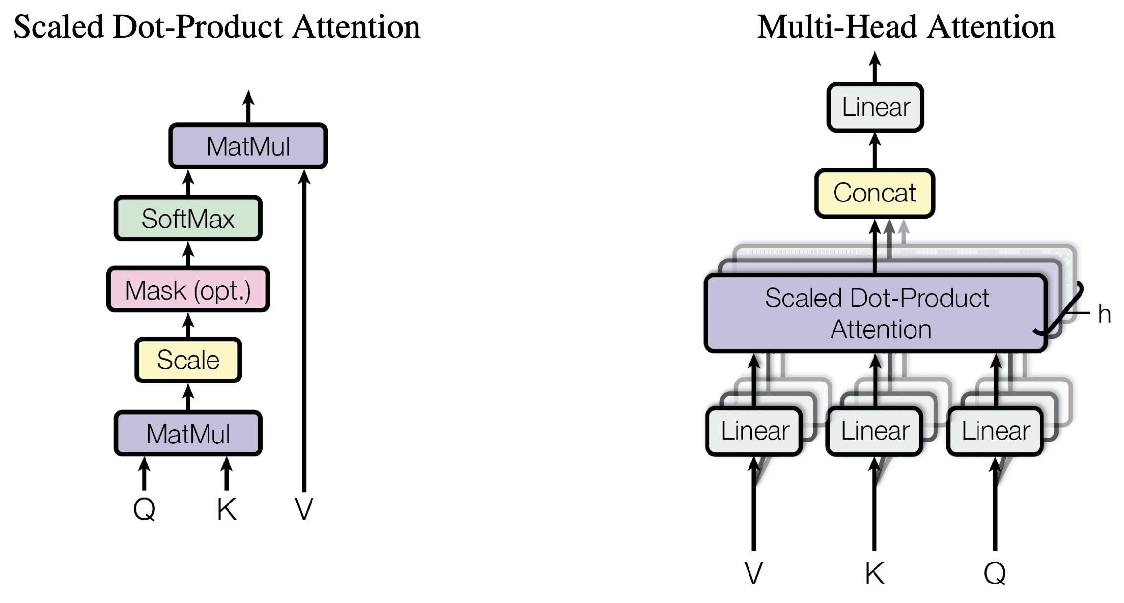
A diagram of the multi-head attention mechanism and the scaled dot-product attention from Vaswani et al.
Specifically we are going to focus on taking an input, creating the keys, queries, and values, and then calculating the scaled dot-product attention. We will not be focusing on the multi-head attention mechanism for our simple example. If you are not familiar with some of these concepts, I recommend watching Andrej Karpathy’s video where he builds a transformer model from scratch and explains the intuition behind each component.
Simple Example
Let’s start with a simple example, much like the one provided by Jinoo Baek. We will start with a sequence of two words, “Hello World”.
Tokenization
For this task we will encode the sequence using the byte-pair encoding (BPE) algorithm used for GPT-2. We can access this using the tiktoken Python package. Let’s start by importing the package and encoding our sequence.
import tiktoken

enc = tiktoken.get_encoding('gpt2')
s = "Hello World"
x = enc.encode(s)
print(x) # [15496, 2159]
The tokenizer takes the sequence and turns it into a list of integers, which is something that the computer can understand.
Token Embedding
Our vocabulary size with the GPT-2 tokenizer is 50257. We could represent our words as one-hot vectors, however they wouldn’t contain any meaningful information in them besides exactly what word or word piece we are referring to. There is no contextual information in this type of representation. We would like to represent these integers rather as vectors of smaller dimensions that contain more information than a 1 in a sea of 0’s. This allows the model to learn more meaningful representations of these tokens or word parts (for a great post on this, check out Lena Voita’s post on Word Embeddings).
For our simple example, we will create embeddings of size 3. We will leverage some PyTorch code to do this for us.
import torch
import torch.nn as nn

tok_emb = nn.Embedding(enc.n_vocab, 3)
et = tok_emb(torch.tensor(x))
Visualizing the embeddings, we can see that they are 2 vectors of size 3.
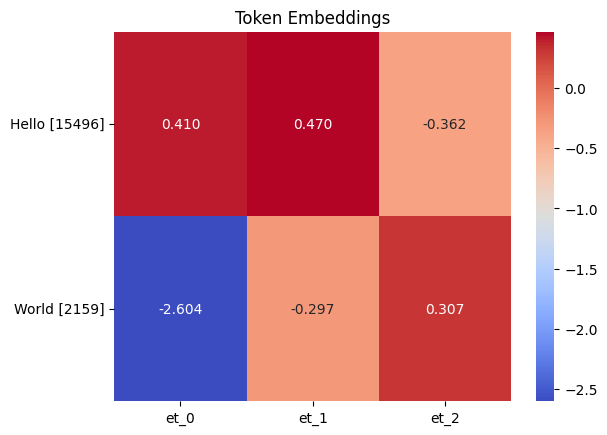
Token embeding of Hello World. Each word is represneted by a vector of size 3.
Position Embedding
Now, we need to represent the position of each token in the sequence. For our simple example, we will create another learnable embedding of size 3.
pos = torch.arange(len(x))
pos_emb = nn.Embedding(2, 3)
ep = pos_emb(pos)
This will similarly be a vector of size 3 for each token in the sequence. The y labels in the following image are the position index of each token in the sequence.
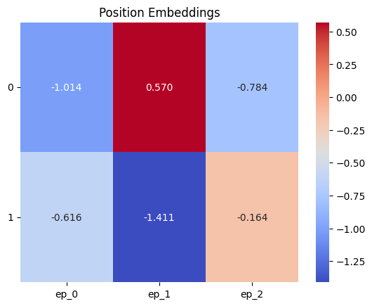
Position embeding of Hello World. Each word is represneted by a vector of size 3.
Combined Embedding
Now we can combine the token and position embeddings to create the input embeddings for our model. We will simply add the two embeddings together.
ec = et + ep
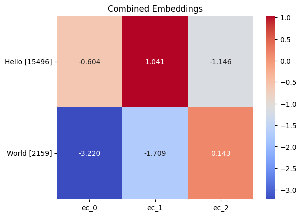
Combined embeding of Hello World. Each word is represneted by a vector of size 3.
Queries, Keys, and Values
Now we can get to meat of the attention mechanism. We will use 3 simple linear layers to create the queries, keys, and values. These are learnable parameters that can be trained eventually. Roughly speaking, the queries represent the word that we are inquiring about, the keys represent the other words in the sequence, and the values represent information that we would like to pass forward in our network regarding each word in the sequence. Let’s create our query, key, and values.
q_wt = nn.Linear(3, 3)
k_wt = nn.Linear(3, 3)
v_wt = nn.Linear(3, 3)
q = q_wt(ec)
k = k_wt(ec)
v = v_wt(ec)
Here is what they look like visualized. Right now, these are random values, but they will be trained later.

Queries, keys, and values for our sequence.
Scaled Masked Causal Attention
Now we can calculate the attention for each word in the sequence using our queries, keys, and values. First we calculate the dot product between the queries and the keys. This is essentially looking at how much each of the words in the sequence should attend to each other.
attn = q @ k.transpose(-1, -2)
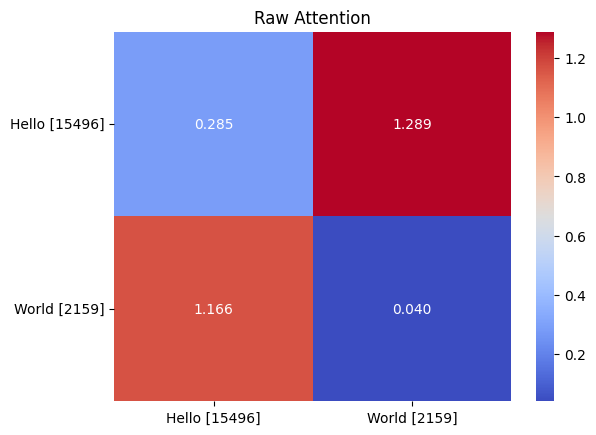
Raw attention values after the dot product.
Right now, these are essentially the logits for how important each input word (y-axis) is to the target word (x-axis) in the sequence.
Now we need to apply a mask to the attention matrix. This mask will be a triangular matrix that will prevent the attention mechanism from attending to future words in the sequence. This is one key to the causal attention mechanism.
mask = torch.tril(torch.ones_like(attn))
attn_masked = attn.masked_fill(mask == 0, float('-inf'))
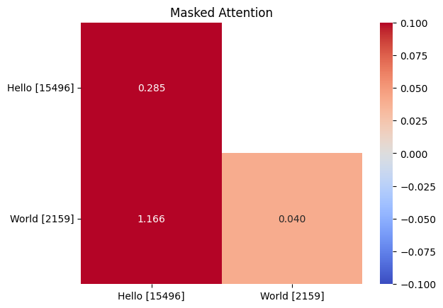
Masked raw attention values. Notice that we cannot attend to the target word of "World" from the input word of "Hello" because we haven't made it that far in the sentence yet.
Lastly, we need to apply the softmax function. First, we will scale the attention values by the square root of the embedding size. This trick normalizes the variance which helps reduce the chance of exploding gradients. Then we apply the softmax function to get the attention weights.
attn_scaled_softmax = F.softmax(attn_masked / np.sqrt(3), dim=-1)
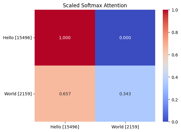
Scaled attention values. Now we can see a little intuition here as the softmax turns the logits into probabilities.
Finally, intuition takes hold here. Each cell represents with what probability the input word (y-axis) should attend to the target word (x-axis). We can see that the input word of “Hello” should attend to itself with a probability of 1.0. This is because it is the first word in the sequence and therefor cannot attend to any other word. However, given our randomly initialized parameters, we can see that “World” should attend to the values of “Hello” slightly more than itself.
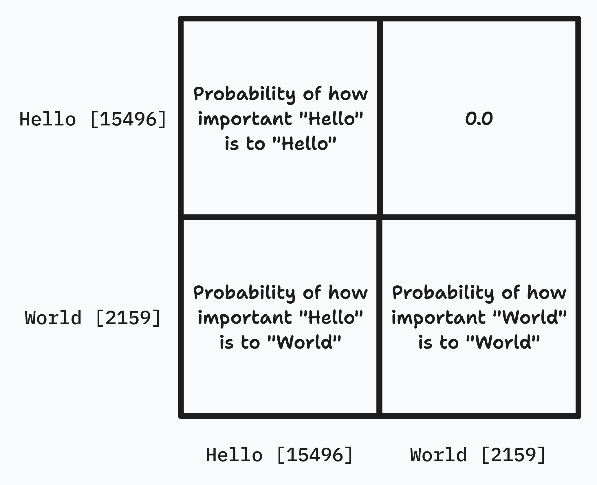
Intuition to the scaled attention attention probabilities. Credit to Jinoo Baek's blog post for this thought.
We can see that the mask ensures that the attention mechanism cannot apply any level of importance to future words. This is another key to the causal attention mechanism.
Weighted Values
Now that we have the probabilities/attention weights, we can scale our values proportionally by the weights. The values are also learnable parameters that will be trained and will contain vital information that allows the model to help predict the next word in the sequence.
weighted_values = attn_scaled_softmax @ v
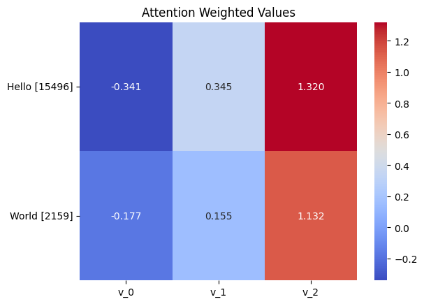
Weighted values. We see that the value vector for 'Hello' did not change, but the value vector for 'World' did as it is a weighted combination of both value vectors.
These weighted combinations of the values are important for the model to learn how to predict the next word in the sequence. It is the weighted combination that allows a model to pay attention to more than one word if needed. Also keep in mind that all the embeddings, and linear layers are learnable parameters that will be trained based on our dataset.
Let’s train it
OK, we now have the building blocks for a very basic transformer model. Let’s put it all together and train it to do one thing, predict “ World” if it is given “Hello”. The following code is a PyTorch module that will make up our model
class HelloWorldModel(nn.Module):
    def __init__(self, n_embd=3):
        super().__init__()
        self.enc = tiktoken.get_encoding('gpt2')
        self.tok_emb = nn.Embedding(self.enc.n_vocab, n_embd)
        self.pos_emb = nn.Embedding(5, n_embd)
        self.q_wt = nn.Linear(n_embd, n_embd, bias=False)
        self.k_wt = nn.Linear(n_embd, n_embd, bias=False)
        self.v_wt = nn.Linear(n_embd, n_embd, bias=False)
        self.out = nn.Linear(n_embd, self.enc.n_vocab, bias=False)

        # storage for inspection
        self.et = None
        self.ep = None
        self.ec = None
        self.q = None
        self.k = None
        self.v = None
        self.attn = None
        self.attn_masked = None
        self.attn_scaled_softmax = None
        self.weighted_values = None

    def forward(self, x):
        B, T = x.shape
        # Embed the tokens
        self.et = self.tok_emb(x) # B, T, C

        # Get the positions
        pos = torch.arange(T)   # T

        # Embed the positions
        self.ep = self.pos_emb(pos) # B, T, C

        # Combine token and position embeddings
        self.ec = self.et + self.ep # B, T, C

        # Create query, key, and values
        self.q = self.q_wt(self.ec) # B, T, C
        self.k = self.k_wt(self.ec) # B, T, C
        self.v = self.v_wt(self.ec) # B, T, C

        # Calculate attention
        self.attn = self.q @ self.k.transpose(-1, -2) # B, T, T

        # Create attention mask
        mask = torch.tril(torch.ones_like(self.attn)) # B, T, T
        self.attn_masked = self.attn.masked_fill(mask == 0, float('-inf')) # B, T, T

        # Scaled Softmax attention
        self.attn_scaled_softmax = F.softmax(self.attn_masked / np.sqrt(3), dim=-1) # B, T, T

        # Calculate the weighted values
        self.weighted_values = self.attn_scaled_softmax @ self.v # B, T, C

        # Calculate the output
        out = self.out(self.weighted_values) # B, T, n_vocab

        return out
You should see almost all the same components that we introduced in the simple example. The only difference is that we are packaging it all up into a PyTorch module. We also added a few lines to store the intermediate values for inspection. Let’s train this model to predict “ World” if it is given “Hello”.
# Data
x = torch.tensor(enc.encode_batch(['Hello World!']))

# Model
model = HelloWorldModel()

# Training loop
max_iters = 1000
log_step = 100
lossi = []
optimizer = torch.optim.SGD(model.parameters(), lr=0.1)

for i in range(max_iters):
    # Forward pass
    xtr = x[:, :-1]
    ytr = x[:, 1:]
    out = model(xtr)

    # Calculate loss
    out = out.view(-1, out.shape[-1])
    ytr = ytr.contiguous().view(-1)
    loss = F.cross_entropy(out, ytr)
    if i % log_step == 0:
        print(f'{i}/{max_iters}: Loss: {loss.item()}')
    lossi.append(loss.item())

    # Backward pass
    optimizer.zero_grad()
    loss.backward()
    optimizer.step()

print(f'{max_iters}/{max_iters}: Loss: {loss.item()}')
1000 steps is a bit overkill, however it is a simple model and it trains very quickly. Here is the loss curve.
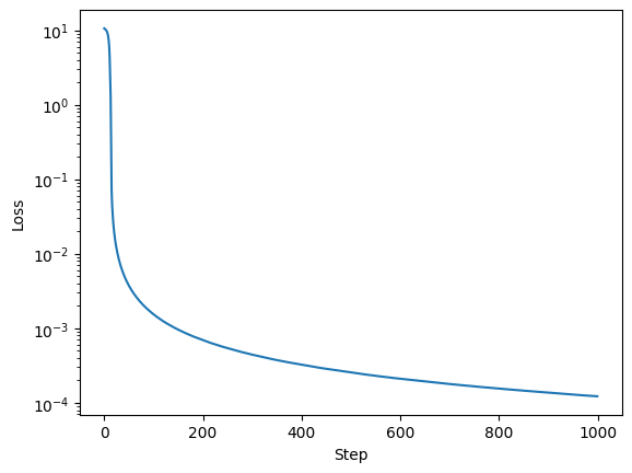
Loss curve for training the basic model.
Now we can predict the next word in the sequence given “Hello”.
new = torch.tensor([enc.encode('Hello')])
print(enc.decode(model(new).argmax(-1).tolist()[0])) # ' World'
Notice that our predicted word has a space in front of “World”. This is because the model has a single token that represents “ World”.
Visualizing the attention
The combined embeddings did not change too drastically during training, however the queries, keys, and values did.

Trained queries, keys, and values.
Compared to the untrained values, we can see that some learning happened. However, it is hard to make any insight from this because we are still dealing with embeddings, which are abstractions that are hard to interpret. Instead, let’s look at the computed attention probabilities.
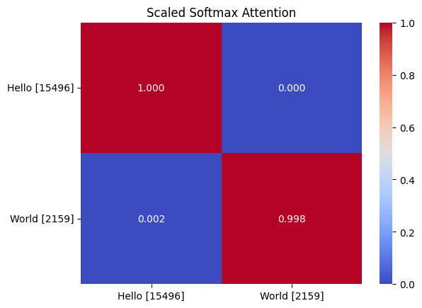
Trained attention probabilities.
OK, here is something. We can clearly see that the model believes that predicting the next word almost solely depends on the current word it is looking at. This makes sense because we trained the model to do one simple task, predict “ World” if it is given “Hello”. This shows a problem with our training data. We only gave the model one example of a sequence. If we gave it more examples, it would learn that the next word in the sequence is not always “ World”. Let’s try that.
Training with more complicated data
Our new data should be a bit more complicated, something that it has to learn how to attend to a specific word in the sequence in order to predict the correct next word. Here is what we will use.
data = [
    'The dog is an animal',
    'The human is a person',
    'The rock is a mineral',
    'The tree is a plant',
    'The car is a vehicle',
    'The sun is a star',
]
For our test, let’s just focus on getting the model to predict the last word in each sentence correctly if given the first 4 words. This means that the model will need to pay attention to the second word in the sequence to make the correct prediction. We will use the same model as before, but we will train it on this new data, and increase its embedding size to 5 in order to capture more meaningful representations of each word/token.
# Encode the data
data_enc = torch.tensor(enc.encode_batch(data))
xtr = data_enc[:, :-1]
ytr = data_enc[:, 1:]

modelv2 = HelloWorldModel(n_embd=5)

# Training loop
max_iters = 10000
log_step = 1000
lossi = []
optimizer = torch.optim.AdamW(modelv2.parameters(), lr=1e-4)

for i in range(max_iters):
    # Forward pass
    xtr = data_enc[:, :-1]
    ytr = data_enc[:, 1:]
    out = modelv2(xtr)

    # Calculate loss
    out = out.view(-1, out.shape[-1])
    ytr = ytr.contiguous().view(-1)
    loss = F.cross_entropy(out, ytr)
    if i % log_step == 0:
        print(f'{i}/{max_iters}: Loss: {loss.item()}')
    lossi.append(loss.item())

    # Backward pass
    optimizer.zero_grad()
    loss.backward()
    optimizer.step()

print(f'{max_iters}/{max_iters}: Loss: {loss.item()}')
This training takes a bit longer because we increased our sequence length and we increased our embedding size. Here is the loss curve.
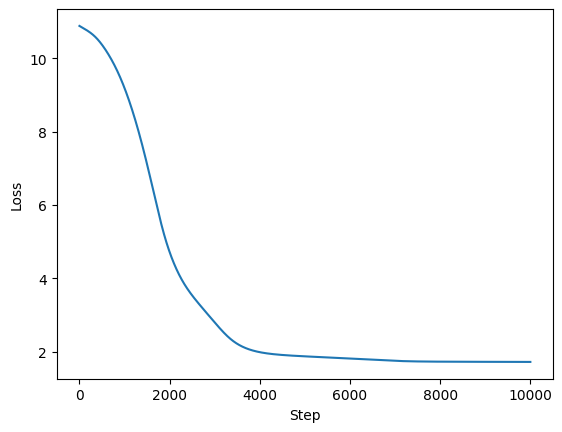
Training loss for the expanded dataset.
Now we can predict the next word in each of the training sequences given the first 4 words.
out = modelv2(xtr)
for i in range(len(xtr)):
    print(enc.decode(out.argmax(-1).tolist()[i][-1:]))

# output
'''
animal
person
mineral
plant
vehicle
star
'''
Visualizing the attention
Now let’s see if there are any more meaningful insights that we can gain from visualizing the parameters.

Trained queries, keys, and values for the more complicated dataset.
Let’s pay attention to the query vector for “a” as it is this vector that will be used to attend to the other words in the sequence to predict the last word. We see that that the magnitude for each of its elements are large in comparison to other query vectors. Furthermore, if you compare the query vector for “a” to the key vectors, we can see that the signs and magnitudes line up well for the key vector for “human”. This makes sense because the model needs to attend to “human” in order to predict “person”. When the queries are matrix multiplied with the keys we get the following attention matrix.
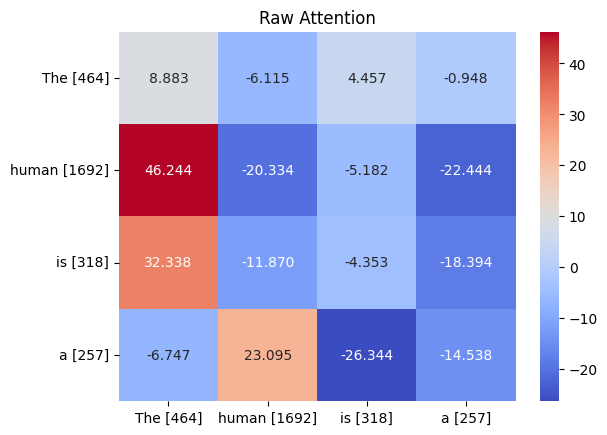
Trained raw attention matrix for the more complicated dataset.
Again, let’s focus on the row for “a”. We can see that the logits are heavily positive for “human”. This supports our observation from the query and key matrices. The story is complete when we observe the resulting attention probabilities/weights.
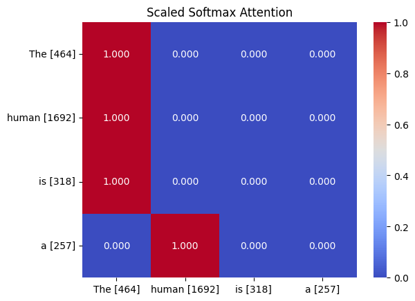
Trained attnetion probabilites/weights for the more complicated dataset.
Now it is clear that the model is paying attention to the second word in the sequence when predicting the last word. This is because for row “a”, the model has a probability of 1.0 for the second word in the sequence. What this will translate to is that the model will pass 100% of the value information from the second word in the sequence to the full-feedforward network to make its prediction, which is what we wanted it to do.
Interestingly, the model also learned to only pay attention to the first word, “The”, when predicting any other word in the sequence. For our purposes, this is fine, but if we wanted the model to learn to predict words in the middle of the sequence, we would need to train it on more examples.
Conclusion
- The more complicated dataset allowed us to see how the attention mechanism can be used to attend to specific words in the sequence.
- This model and dataset is grossly oversimplified, but it helped me understand the intuition behind the attention mechanism.
- With this, we should be able to imagine how scaling the sequence length, embedding size, and size of other the other parameters can help the model attend to more than one word in the sequence.
- Furthermore, with multiple attention heads or multiple layers, the model can attend to more complicated relationship between these words as well.
- Lastly, training the model on a more complicated dataset will allow the model to learn more complicated relationships between the words in the sequence.
- Play around with this code!
Enjoy Reading This Article?
Here are some more articles you might like to read next: